From equations of state to gravitational wave spectra
Mika Mäki, Doctoral Researcher,
Computational Field Theory group, University of Helsinki
Advancing gravitational wave predictions from cosmological first-order phase transitions
CERN, 28.8.2025
Different types of phase transition simulations
- Lattice simulations
- Capture multiple types of effects: bubble expansion, collision and turbulence
- Computationally expensive
- Analytical approximations
- Broken power law, double broken power law
- Useful but rather crude approximations
- Semi-analytical approximation: Sound Shell Model
- Captures dependence on phase transition parameters
- Reproduces the results of lattice simulations for intermediate-strength transitions
Self-similar fluid shells

Source:
Hindmarsh et al. (2021,
arXiv:2008.09136),
hybrids discovered by Kurki-Suonio & Laine (1995,
arXiv:hep-ph/9501216)
Friction → constant $v_\text{wall}$ → self-similar solution
Three types of solutions, determined by
Three types of solutions, determined by
- Wall velocity $v_\text{wall}$
- Transition strength $\alpha_n$
- Speed of sound $c_s(T,\phi)$
Explanation of the figure
- Black circle: phase boundary, aka. bubble wall
- Colour: velocity of moving plasma
- $c_s$: speed of sound
- $v_\text{w}$: wall speed
- $c_\text{J}$: Chapman-Jouguet speed
Equations of state
- Equation of state for an ultrarelativistic plasma with multiple degrees of freedom $$p(T,\phi) = \frac{\pi^2}{90} g_p(T,\phi) T^4 - V(T,\phi)$$
-
The rest can be deduced with thermodynamics
-
Entropy density $s = \frac{dp}{dT}$,
enthalpy density $w = Ts$,
energy density $e = w - p$, sound speed $c_s \equiv \sqrt{\frac{dp}{de}}$
-
Entropy density $s = \frac{dp}{dT}$,
enthalpy density $w = Ts$,
- Bag model: equation of state with constant degrees of freedom $$p_\pm = a_\pm T^4 - V_\pm \quad \Rightarrow \quad c_s^2 \equiv \frac{dp}{de} = \frac{1}{3}$$
-
Constant sound speed model
(aka. $\mu, \nu$ model or template model, arXiv:2004.06995, arXiv:2010.09744) $$p_\pm = a_\pm \left( \frac{T}{T_0} \right)^{\mu_\pm - 4} T^4 - V_\pm {\color{gray} \approx a_\pm T^{\mu_\pm} - V_\pm } \quad \Rightarrow \quad c_{s\pm}^2 = \frac{1}{\mu_\pm - 1}$$ -
From an arbitrary particle physics model: $g_p(T,\phi), \ V(T,\phi)$
- This can also be done with e.g. WallGo (arXiv:2411.04970)

Sound Shell Model
- Hindmarsh (2018, arXiv:1608.04735), Hindmarsh & Hijazi (2019, arXiv: 1909.10040)
-
When the transition strength $\alpha_n \ll 1$ and $v_\text{wall} < 1$
- Sound waves are the majority contribution
→ collisions and turbulence can be neglected → no interaction between the bubbles
- Sound waves are the majority contribution

Correction factors
-
Giombi et al. (2024, arXiv:2409.01426):
Changing the sound speed → source lifetime factor $\Lambda$
$$\begin{align} \tilde{P}_\text{gw,corr.}(k) &\equiv \Lambda \tilde{P}_\text{gw}(k) & \Lambda &\equiv \frac{1}{1 + 2\nu} \left(1 - \left(1 + \frac{\Delta \eta}{\eta_*} \right) \right)^{-1-2\nu} \\ \nu_\text{gdh2024} &\equiv \frac{1-3\omega}{1 + 3\omega} & \omega(T,\phi) &\equiv \frac{p(T,\phi)}{e(T,\phi)} \quad \textcolor{gray}{\omega_\text{bag} = \frac{1}{3} \rightarrow \nu_\text{bag} = 0} \end{align}$$ -
Gowling & Hindmarsh (2021, arXiv:2106.05984): Suppression factor
- From comparison with 3D hydrodynamic simulations
-
Giombi et al. (2024, arXiv:2409.01426)
- Low-frequency tail of the spectrum
 Suppression factor
 Low-frequency tail
PTtools: From equations of state to GW spectra
- Python-based simulation framework, doi:10.5281/zenodo.15268219
-
Based on the Sound Shell Model by Hindmarsh et al.
- Computationally efficient compared to lattice simulations
- Developed by Mark Hindmarsh, Chloe Hopling (f.k.a. Gowling), Mika Mäki & Lorenzo Giombi
-
Input
- Equation of state: $p(T,\phi)$
- Wall speed $v_\text{wall}$
- Transition strength parameter $\alpha_n \equiv \frac{4D\theta(T_n)}{3w_n} = \frac{4}{3} \frac{\theta_+(T_n) - \theta_-(T_n)}{w_n}$
- Hubble-scaled mean bubble spacing $r_* \equiv H_n R_*$
- Output: GW power spectrum today $\Omega_{gw,0}(f)$
- Use case: estimate the likelihood of various Standard Model extensions with LISA data

From fluid profiles to GW spectra

🠮

Fluid shell velocity profiles
- Boundary conditions
- ODE integration
GW spectra
- Sound Shell Model: sine transform etc.
- Conversion to observable $f$ etc.
- Experimentally testable by LISA
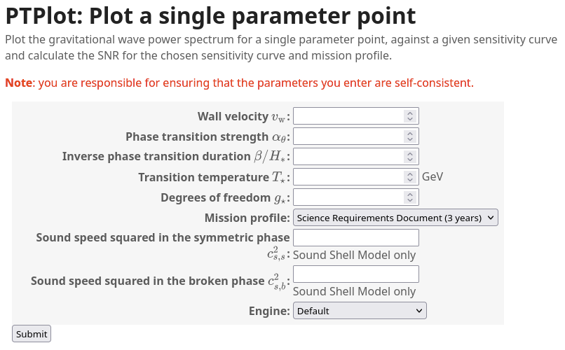
PTPlot: Easy plotting of GW spectra
-
Online plotting utility, arXiv:1704.05871
- Based on the Python web framework Django
- Developed by David Weir, Deanna Hooper, Jenni Häkkinen & Mika Mäki
-
Supports several models for the GW spectrum
- Broken power law
- Double broken power law (upcoming)
- Sound Shell Model (upcoming)
Summary
- The equation of state has a significant effect on the GW spectrum
- Sound Shell Model enables quick computation of the GW spectrum
- Utilities: PTtools & PTPlot, https://www.ptplot.org
- Open question: How sensitive will LISA be to different sound speeds?
Fluid velocity profiles

Fluid velocity profiles

GW power spectra

GW power spectra

GW power spectra today

GW power spectra today
