Generating gravitational wave spectra from phase transitions with realistic equations of state

Mika Mäki, Doctoral Researcher,
Computational Field Theory group, University of Helsinki

8.8.2025

Contents of the talk

• Introduction: Types of simulations
• Hydrodynamics
  • Dimensionality of the problem
  • Wave equation
  • Phase boundary
  • Hydrodynamic equations
  • Fluid shell types
• Equations of state
• Sound Shell Model
  • Correction factors
• Simulation software
  • PTtools
  • PTPlot

Dimensionality of the problem

• We investigate the expansion of a single bubble
• Self-similarity
  • Friction results in a constant wall speed $v_\text{wall}$
  • As the bubble expands, its relative shape stays the same
  • → Time-independent solution
• Spherical symmetry
• 3+1 dimensional problem reduces to time-independent 1D

Wave equation

• Constant background space-time → energy-momentum conservation $\nabla_\mu T^{\mu\nu} = 0$
• Energy-momentum tensor of an ideal fluid $$T^{\mu \nu}_f = (e+p) u^\mu u^\nu + p g^{\mu \nu}$$
• For a one-dimensional flow in Cartesian coordinates $$\begin{align} \partial_t \left[ (e+pv^2) \gamma^2 \right] + \partial_x \left[ (e+p) \gamma^2 v \right] &= 0, \label{eq:ep_conservation_1d_1} \\ \partial_t \left[ (e+p) \gamma^2 v \right] + \partial_x \left[ (ev^2 + p) \gamma^2 \right] &= 0 \label{eq:ep_conservation_1d_2} \end{align}$$
• First-order perturbation → wave equation with a speed of sound $$\partial_t^2 (\delta e) - \frac{\delta p}{\delta e} \partial_x^2(\delta e) = 0 \qquad c_s^2 \equiv \frac{dp}{de} = \frac{dp/dT}{de/dT}$$

Phase boundary

• Energy-momentum conservation $$\nabla_\mu T^{\mu\nu} = 0 \quad \Rightarrow \quad \partial_z T^{zz} = \partial_z T^{z0} = 0$$
• Inserting ideal fluid $T^{\mu \nu}_f = (e+p) u^\mu u^\nu + p g^{\mu \nu}$ → junction conditions $$\begin{align} w_- \tilde{\gamma}_-^2 \tilde{v}_- &= w_+ \tilde{\gamma}_+^2 \tilde{v}_+ \label{eq:junction_condition_1} \\ w_- \tilde{\gamma}_-^2 \tilde{v}_-^2 + p_- &= w_+ \tilde{\gamma}_+^2 \tilde{v}_+^2 + p_+ \label{eq:junction_condition_2} \end{align}$$
• By defining new variables $\theta = \frac{1}{4}(e-3p), \quad \textcolor{red}{\alpha_+} \equiv \frac{4}{3} \frac{\theta_+(w_+) - \theta_-(w_-)}{w_+}$ $$\begin{align} \tilde{v}_+ &= \frac{1}{2(1+\textcolor{red}{\alpha_+})}\left[ \left(\frac{1}{3\tilde{v}_-}+\tilde{v}_-\right) \pm \sqrt{\left(\frac{1}{3\tilde{v}_-} - \tilde{v}_- \right)^2 + 4\textcolor{red}{\alpha_+}^2 + \frac{8}{3} \textcolor{red}{\alpha_+}} \right], \label{eq:v_tilde_plus} \\ \tilde{v}_- &= \frac{1}{2} \left[ \left( (1+\textcolor{red}{\alpha_+})\tilde{v}_+ + \frac{1-3\textcolor{red}{\alpha_+}}{3\tilde{v}_+} \right) \pm \sqrt{\left((1+\textcolor{red}{\alpha_+})\tilde{v}_+ + \frac{1-3\textcolor{red}{\alpha_+}}{3\tilde{v}_+} \right)^2 - \frac{4}{3}} \right]. \label{eq:v_tilde_minus} \end{align}$$

Hydrodynamic equations

• Energy-momentum conservation $\nabla_\mu T^{\mu\nu} = 0$
• Projection → hydrodynamic equations away from the phase boundary $$\begin{align} 0 &= u_\mu \partial_\nu T^{\mu \nu} = -\partial_\mu (w u^\mu) + u^\mu \partial_\mu p, \\ 0 &= \bar{u}_\mu \partial_\nu T^{\mu \nu} = w \bar{u}^\nu u^\mu \partial_\mu u_\nu + \bar{u}^\mu \partial_\mu p. \end{align}$$
• Using self-similarity $\xi = \frac{r}{t}$ and parametrising $$\begin{align} \frac{d\xi}{d\tau} &= \xi \left[ (\xi - v)^2 - c_s^2 (1 - \xi v)^2 \right], \\ \frac{dv}{d\tau} &= 2 v c_s^2 (1 - v^2) (1 - \xi v), \\ \frac{dw}{d\tau} &= w \left( 1 + \frac{1}{c_s^2} \right) \gamma^2 \mu \frac{dv}{d\tau}. \end{align}$$
• Note that $c_s^2$ is computed using user-provided functions

Fluid shells

General equation of state

• Equation of state for an ultrarelativistic plasma with multiple degrees of freedom $$p(T,\phi) = \frac{\pi^2}{90} g_p(T,\phi) T^4 - V(T,\phi)$$
• The rest can be deduced with thermodynamics
  • Entropy density $s = \frac{dp}{dT}$
  • Enthalpy density $w = Ts$
  • Energy density $e = w - p$
  • Sound speed $c_s \equiv \sqrt{\frac{dp}{de}}$

Simple equations of state

• Bag model: equation of state with constant degrees of freedom $$g_\pm = \frac{90}{\pi^2} a_\pm \quad \Rightarrow \quad p_\pm = a_\pm T^4 - V_\pm, \quad c_s^2 \equiv \frac{dp}{de} = \frac{1}{3}$$
• Constant sound speed model (aka. $\mu, \nu$ model or template model) $$\begin{align} g_{p\pm} &= \frac{90}{\pi^2} a_\pm \left( \frac{T}{T_0} \right)^{\mu_\pm - 4} \\ \Rightarrow \quad p_\pm &= a_\pm \left( \frac{T}{T_0} \right)^{\mu_\pm - 4} T^4 - V_\pm {\color{gray} \approx a_\pm T^{\mu_\pm} - V_\pm } \\ c_{s\pm}^2 &= \frac{1}{\mu_\pm - 1} \end{align}$$

Equation of state from an arbitrary particle physics model

• Non-constant degrees of freedom → varying speed of sound $c_s(T,\phi)$
• The equation of state can be constructed from $V(T,\phi), \ g_p(T,\phi)$ and preferably also $g_e(T,\phi)$ or $g_s(T,\phi)$ $$\begin{align} g_p &= 4g_s - 3g_e \\ e(T,\phi) &= \frac{\pi^2}{30} g_e(T,\phi) T^4 + V(T, \phi) \\ p(T,\phi) &= \frac{\pi^2}{90} g_p(T,\phi) T^4 - V(T, \phi) \\ s(T,\phi) &= \frac{2\pi^2}{45} g_s(T,\phi) T^3 \end{align}$$
• This can also be done with e.g. WallGo

Sound Shell Model

• Hindmarsh (2018), Hindmarsh & Hijazi (2019)
• When the transition strength $\alpha_n \ll 1$ and $v_\text{wall} < 1$
  • Sound waves are the majority contribution: $\Omega_{gw} = \textcolor{gray}{\Omega_{collisions}} + \Omega_{sw} + \textcolor{gray}{\Omega_{turbulence}}$
  • Collisions and turbulence can be neglected → no interaction between the bubbles
• After the bubbles have merged, the fluid shells continue as sound waves
• The velocity field is the superposition of the individual bubbles that have $v(\xi), e(\xi), w(\xi)$
• Sine transformation to wavenumber space → wavefunction launched by a single bubble $A(z)$
• Superposition of bubbles → plane wave components of the velocity field $P_v(z)$
• Shear stress in the fluid → unequal time correlator (UETC) of the shear stress, $U_\Pi$
• → GW power spectrum $\mathcal{P}_{gw}(z)$
• Conversion from $z$ to $f$: $\mathcal{P}_{gw}(z)$ → $\Omega_{gw,0}(f)$
• Together: $(v(\xi), e(\xi), w(\xi)) \rightarrow A(z) \rightarrow P_v \rightarrow U_\pi \rightarrow \mathcal{P}_{gw}(z) \rightarrow \Omega_{gw,0}(f)$

Correction factors

PTtools: From equations of state to GW spectra

• Python-based simulation framework
• Based on the Sound Shell Model by Hindmarsh et al.
  • Computationally efficient compared to lattice simulations
• Developed by Mark Hindmarsh, Chloe Hopling & Mika Mäki
• Input
  • Equation of state: $p(T,\phi)$
  • Wall speed $v_\text{wall}$
  • Transition strength parameter $\alpha_n \equiv \frac{4D\theta(T_n)}{3w_n} = \frac{4}{3} \frac{\theta_+(T_n) - \theta_-(T_n)}{w_n}$
  • Hubble-scaled mean bubble spacing $r_* \equiv H_n R_*$
• Output: GW power spectrum today $\Omega_{gw,0}(f)$
• Use case: estimate the likelihood of various Standard Model extensions with LISA data

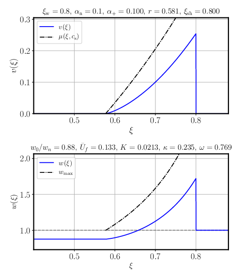
Fluid shell algorithm: detonations

• Solve boundary conditions at the wall for known $w_+=w_n, v_+=0$
  • Using user-provided $p(T,\phi)$ → numerical solving
• Integrate from the wall to the fixed point at $v=0$
  • Using $c_s^2(w,\phi)$ based on user-provided functions → numerical ODE integration

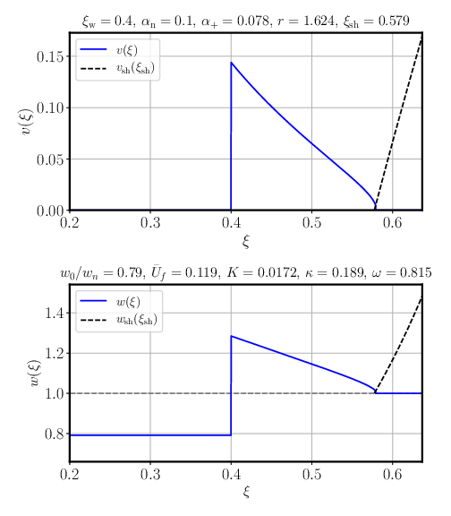
Fluid shell algorithm: deflagrations

• Guess $w_-$, the enthalpy behind the wall
• Solve boundary conditions at the wall for $w_+, v_+$
• Integrate to the shock
  • $v_{sh}(\xi)$ is computed from the boundary conditions → has to be found numerically
• Solve boundary conditions at the shock
• Check if $w=w_n$
• If not, change the enthalpy guess and try again

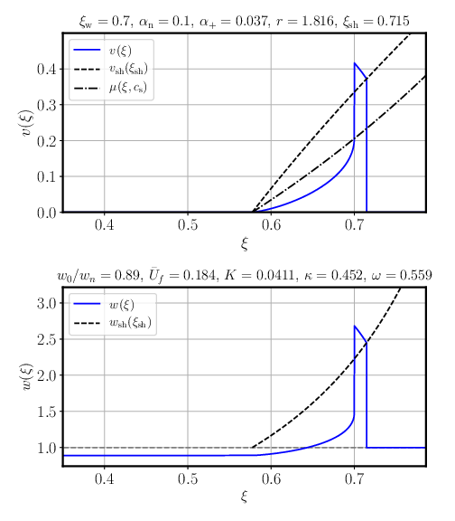
Fluid shell algorithm: hybrids

• The same as for subsonic deflagrations, but with an additional integration behind the wall
• Guess $w_-$, the enthalpy behind the wall
• Solve boundary conditions at the wall for $w_+, v_+$
• Integrate to the shock
• Solve boundary conditions at the shock
• Check if $w=w_n$
• If not, change the enthalpy guess and try again
• Once the correct enthalpy has been found, integrate from the wall to the fixed point at $v=0$

From fluid profiles to GW spectra

🠮

Fluid shell velocity profiles

• Boundary conditions
• ODE integration

GW spectra

• Sine transform
• Conversion to observable $f$ etc.
• Experimentally testable by LISA

How to use PTtools

                        pip install pttools-gw
                    

                            
                                from pttools.analysis import plot_spectra_omgw0, plot_bubbles_v
                                from pttools.bubble import Bubble
                                from pttools.models import ConstCSModel
                                from pttools.omgw0 import Spectrum

                                alpha_n = 0.2
                                model = ConstCSModel(css2=1/3, csb2=1/4, alpha_n_min=alpha_n)
                                bubbles = [
                                    Bubble(model, v_wall=0.3, alpha_n=alpha_n),
                                    Bubble(model, v_wall=0.5, alpha_n=alpha_n),
                                    Bubble(model, v_wall=0.9, alpha_n=alpha_n)
                                ]
                                spectra = [Spectrum(bubble, r_star=0.1, Tn=200) for bubble in bubbles]

                                plot_bubbles_v(bubbles, path="bubbles.svg", v_max=0.5)
                                plot_spectra_omgw0(spectra, path="spectra.svg")
                            
                        

https://pttools.readthedocs.io

Fluid velocity profiles

Fluid velocity profiles

GW power spectra

GW power spectra

GW power spectra today

GW power spectra today

PTPlot: Easy plotting of GW spectra

https://ptplot.org