Generating gravitational wave spectra from equations of state for phase transitions in the early universe

Mika Mäki, Doctoral Researcher,
Computational Field Theory group, University of Helsinki

Physics Days
6.3.2026

In collaboration with David Weir, Mark Hindmarsh, Deanna Hooper & Lorenzo Giombi

Online slides

Phase transitions in the early universe

• First-order: potential barrier
  ⇒ phase boundary ⇒ bubble nucleation
• SM Higgs: crossover, BSM Higgs: first-order
  ⇒ Experimental testing of BSM theories

Self-similar fluid shells

From fluid profiles to GW spectra

🠮

Fluid shell velocity profiles

• Boundary conditions
• ODE integration

GW spectra

• Sound Shell Model: sine transform etc.
• Conversion to observable $f$ etc.
• Experimentally testable by LISA

PTtools & PTPlot

https://www.ptplot.org

Signal-to-noise ratio (SNR) with different simulation models

Broken power law (BPL)

Double broken power law (DBPL)

Sound Shell Model (SSM)

• Example particle physics model: Singlet scalar
  • SM extended with a general real singlet scalar field $S$
    $$ \Delta V = b_1 S + \frac{1}{2} b_2 S^2 + \frac{1}{2} a_1 S \left| H \right|^2 + \frac{1}{2} a_2 S^2 \left| H \right|^2 + \frac{1}{3} b_3 S^3 + \frac{1}{4} b_4 S^4 $$
  • SNR curves plotted with $v_\text{wall} = 0.95, T_* = 50.0 \ \text{GeV}, g_* = 107.75$
  • Example points sampled from the parameter space of the model
• Significant change in the shape of the SNR curves with improved simulations

Thank you!

Fluid velocity profiles

Fluid velocity profiles

GW power spectra

GW power spectra

GW power spectra today

GW power spectra today

Equations of state

Sound Shell Model

• Hindmarsh (2018, arXiv:1608.04735), Hindmarsh & Hijazi (2019, arXiv: 1909.10040)
• When the transition strength $\alpha_n \ll 1$ and $v_\text{wall} < 1$
  • Sound waves are the majority contribution
    → collisions and turbulence can be neglected → no interaction between the bubbles

Correction factors

How to use PTtools

                        pip install pttools-gw
                    

                            
                                from pttools.analysis import plot_spectra_omgw0, plot_bubbles_v
                                from pttools.bubble import Bubble
                                from pttools.models import ConstCSModel
                                from pttools.omgw0 import Spectrum

                                alpha_n = 0.2
                                model = ConstCSModel(css2=1/3, csb2=1/4, alpha_n_min=alpha_n)
                                bubbles = [
                                    Bubble(model, v_wall=0.3, alpha_n=alpha_n),
                                    Bubble(model, v_wall=0.5, alpha_n=alpha_n),
                                    Bubble(model, v_wall=0.9, alpha_n=alpha_n)
                                ]
                                spectra = [Spectrum(bubble, r_star=0.1, Tn=200) for bubble in bubbles]

                                plot_bubbles_v(bubbles, path="bubbles.svg", v_max=0.5)
                                plot_spectra_omgw0(spectra, path="spectra.svg")
                            
                        

https://pttools.readthedocs.io

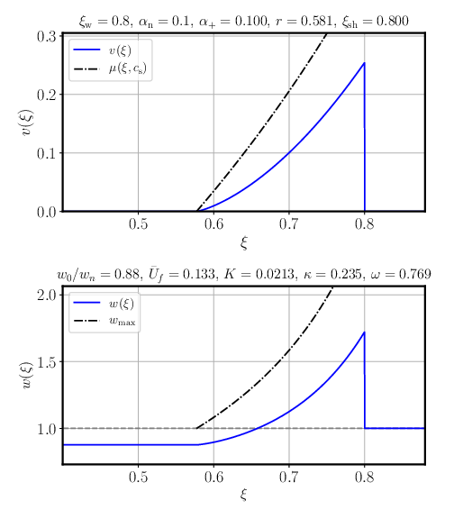
Fluid shell algorithm: detonations

• Solve boundary conditions at the wall for known $w_+=w_n, v_+=0$
  • Using user-provided $p(T,\phi)$ → numerical solving
• Integrate from the wall to the fixed point at $v=0$
  • Using $c_s^2(w,\phi)$ based on user-provided functions → numerical ODE integration

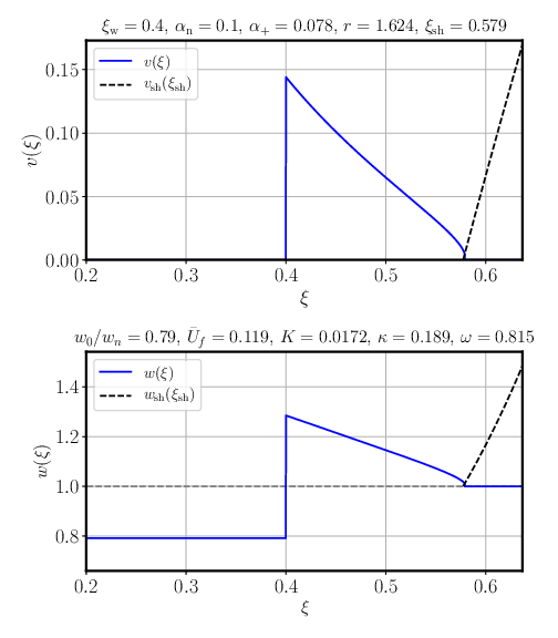
Fluid shell algorithm: deflagrations

• Guess $w_-$, the enthalpy behind the wall
• Solve boundary conditions at the wall for $w_+, v_+$
• Integrate to the shock
  • $v_{sh}(\xi)$ is computed from the boundary conditions → has to be found numerically
• Solve boundary conditions at the shock
• Check if $w=w_n$
• If not, change the enthalpy guess and try again

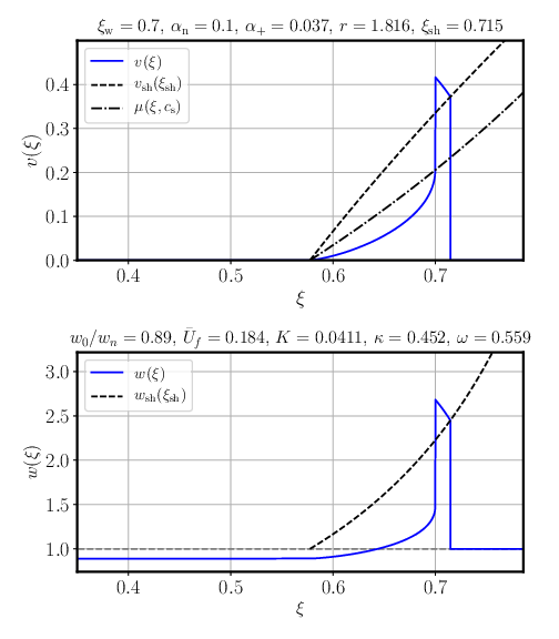
Fluid shell algorithm: hybrids

• The same as for subsonic deflagrations, but with an additional integration behind the wall
• Guess $w_-$, the enthalpy behind the wall
• Solve boundary conditions at the wall for $w_+, v_+$
• Integrate to the shock
• Solve boundary conditions at the shock
• Check if $w=w_n$
• If not, change the enthalpy guess and try again
• Once the correct enthalpy has been found, integrate from the wall to the fixed point at $v=0$

General equation of state

• Equation of state for an ultrarelativistic plasma with multiple degrees of freedom $$p(T,\phi) = \frac{\pi^2}{90} g_p(T,\phi) T^4 - V(T,\phi)$$
• The rest can be deduced with thermodynamics
  • Entropy density $s = \frac{dp}{dT}$
  • Enthalpy density $w = Ts$
  • Energy density $e = w - p$
  • Sound speed $c_s \equiv \sqrt{\frac{dp}{de}}$

Simple equations of state

• Bag model: equation of state with constant degrees of freedom $$g_\pm = \frac{90}{\pi^2} a_\pm \quad \Rightarrow \quad p_\pm = a_\pm T^4 - V_\pm, \quad c_s^2 \equiv \frac{dp}{de} = \frac{1}{3}$$
• Constant sound speed model (aka. $\mu, \nu$ model or template model) $$\begin{align} g_{p\pm} &= \frac{90}{\pi^2} a_\pm \left( \frac{T}{T_0} \right)^{\mu_\pm - 4} \\ \Rightarrow \quad p_\pm &= a_\pm \left( \frac{T}{T_0} \right)^{\mu_\pm - 4} T^4 - V_\pm {\color{gray} \approx a_\pm T^{\mu_\pm} - V_\pm } \\ c_{s\pm}^2 &= \frac{1}{\mu_\pm - 1} \end{align}$$

Equation of state from an arbitrary particle physics model

• Non-constant degrees of freedom → varying speed of sound $c_s(T,\phi)$
• The equation of state can be constructed from $V(T,\phi), \ g_p(T,\phi)$ and preferably also $g_e(T,\phi)$ or $g_s(T,\phi)$ $$\begin{align} g_p &= 4g_s - 3g_e \\ e(T,\phi) &= \frac{\pi^2}{30} g_e(T,\phi) T^4 + V(T, \phi) \\ p(T,\phi) &= \frac{\pi^2}{90} g_p(T,\phi) T^4 - V(T, \phi) \\ s(T,\phi) &= \frac{2\pi^2}{45} g_s(T,\phi) T^3 \end{align}$$
• This can also be done with e.g. WallGo

Wave equation

• Constant background space-time → energy-momentum conservation $\nabla_\mu T^{\mu\nu} = 0$
• Energy-momentum tensor of an ideal fluid $$T^{\mu \nu}_f = (e+p) u^\mu u^\nu + p g^{\mu \nu}$$
• For a one-dimensional flow in Cartesian coordinates $$\begin{align} \partial_t \left[ (e+pv^2) \gamma^2 \right] + \partial_x \left[ (e+p) \gamma^2 v \right] &= 0, \label{eq:ep_conservation_1d_1} \\ \partial_t \left[ (e+p) \gamma^2 v \right] + \partial_x \left[ (ev^2 + p) \gamma^2 \right] &= 0 \label{eq:ep_conservation_1d_2} \end{align}$$
• First-order perturbation → wave equation with a speed of sound $$\partial_t^2 (\delta e) - \frac{\delta p}{\delta e} \partial_x^2(\delta e) = 0 \qquad c_s^2 \equiv \frac{dp}{de} = \frac{dp/dT}{de/dT}$$

Phase boundary

• Energy-momentum conservation $$\nabla_\mu T^{\mu\nu} = 0 \quad \Rightarrow \quad \partial_z T^{zz} = \partial_z T^{z0} = 0$$
• Inserting ideal fluid $T^{\mu \nu}_f = (e+p) u^\mu u^\nu + p g^{\mu \nu}$ → junction conditions $$\begin{align} w_- \tilde{\gamma}_-^2 \tilde{v}_- &= w_+ \tilde{\gamma}_+^2 \tilde{v}_+ \label{eq:junction_condition_1} \\ w_- \tilde{\gamma}_-^2 \tilde{v}_-^2 + p_- &= w_+ \tilde{\gamma}_+^2 \tilde{v}_+^2 + p_+ \label{eq:junction_condition_2} \end{align}$$
• By defining new variables $\theta = \frac{1}{4}(e-3p), \quad \textcolor{red}{\alpha_+} \equiv \frac{4}{3} \frac{\theta_+(w_+) - \theta_-(w_-)}{w_+}$ $$\begin{align} \tilde{v}_+ &= \frac{1}{2(1+\textcolor{red}{\alpha_+})}\left[ \left(\frac{1}{3\tilde{v}_-}+\tilde{v}_-\right) \pm \sqrt{\left(\frac{1}{3\tilde{v}_-} - \tilde{v}_- \right)^2 + 4\textcolor{red}{\alpha_+}^2 + \frac{8}{3} \textcolor{red}{\alpha_+}} \right], \label{eq:v_tilde_plus} \\ \tilde{v}_- &= \frac{1}{2} \left[ \left( (1+\textcolor{red}{\alpha_+})\tilde{v}_+ + \frac{1-3\textcolor{red}{\alpha_+}}{3\tilde{v}_+} \right) \pm \sqrt{\left((1+\textcolor{red}{\alpha_+})\tilde{v}_+ + \frac{1-3\textcolor{red}{\alpha_+}}{3\tilde{v}_+} \right)^2 - \frac{4}{3}} \right]. \label{eq:v_tilde_minus} \end{align}$$

Hydrodynamic equations

• Energy-momentum conservation $\nabla_\mu T^{\mu\nu} = 0$
• Projection → hydrodynamic equations away from the phase boundary $$\begin{align} 0 &= u_\mu \partial_\nu T^{\mu \nu} = -\partial_\mu (w u^\mu) + u^\mu \partial_\mu p, \\ 0 &= \bar{u}_\mu \partial_\nu T^{\mu \nu} = w \bar{u}^\nu u^\mu \partial_\mu u_\nu + \bar{u}^\mu \partial_\mu p. \end{align}$$
• Using self-similarity $\xi = \frac{r}{t}$ and parametrising $$\begin{align} \frac{d\xi}{d\tau} &= \xi \left[ (\xi - v)^2 - c_s^2 (1 - \xi v)^2 \right], \\ \frac{dv}{d\tau} &= 2 v c_s^2 (1 - v^2) (1 - \xi v), \\ \frac{dw}{d\tau} &= w \left( 1 + \frac{1}{c_s^2} \right) \gamma^2 \mu \frac{dv}{d\tau}. \end{align}$$
• Note that $c_s^2$ is computed using user-provided functions